Assignment 6 Solutions: Vector Operations

We want to begin to assess the role of distance from schools in determining the education outcomes for Idahoans. We’ll use the landmarks_pnw.csv and cejst_pnw.shp datasets as the basis for this assignment. You’ll need to load the csv and convert it to an sf object. We want to compare the percentage of individuals age 25 or over with less than a high school degree (HSEF in the cejst dataset) for of counties within 50km of a school (MTFCC == K2543) to those that are more than 50km.

You’ll need to follow many of the same operations in the video example from class. Your assignment is:

1. Write out the pseudocode for your analysis

We’ll need to do a few things here including load the data, find the tracts within 50km of a school, and then compare the cejst results. Breaking that into pseudocode would look like:

1. Load each dataset
2. Subset to schools
3. Check geometry validity
4. Align CRS
5. Find tracts within 50km
6. Make Maps

Note that my fift step (find tracts within 50km) is a little vague. There are lots of ways I could do this. It might be more helpful to add some specificity here like:

1. Load each dataset
2. Subset to schools
3. Check geometry validity
4. Align CRS
5. Buffer schools by 50km
6. Select tracts within the buffer and attribute
7. Make Maps

There are other ways to do this too (like calculating the distance), but those are likely to be more computationally intensive so I’ll leave it at this.

2. Translate the pseudocode into code chunks and create the necessary code (You’ll need to use things like st_distance, st_buffer, st_sym_difference)

Loading the data should be pretty straightforward for you by now. We use read_sf for the shapefile and read_csv for the landmarks.csv. We then filter the data here so that we aren’t working with the entire landmarks dataset.

library(sf)
library(tidyverse, quietly = TRUE)
library(tmap, quietly = TRUE)
cejst.pnw <- read_sf("data/opt/data/2023/assignment06/cejst_pnw.shp")
landmarks.pnw <- read_csv("data/opt/data/2023/assignment06/landmarks_pnw.csv") %>% 
  filter(., MTFCC == "K2543")

We know that one of the datasets are still in long/lat form so we’ll need to make it a sf object before checking the geometry makes any sense. We’ll also assign the crs here by adding it to the st_as_sf call. We also need to make sure that there aren’t any empty geometries as that will cause problems for mapping later.

landmarks.sf <- landmarks.pnw %>% 
  st_as_sf(., coords = c("longitude", "latitude"), crs=4269)
all(st_is_valid(cejst.pnw))

[1] TRUE

all(st_is_valid(landmarks.sf))

[1] TRUE

any(st_is_empty(cejst.pnw))

[1] TRUE

any(st_is_empty(landmarks.sf))

[1] FALSE

Looks like all the geometries are valid, but there are some empty geometries in the cejst dataset. We will drop those by using filter combined with the negation operator (!) and st_is_empty to return the rows where st_is_empty is not equal to TRUE. Then we can move forward with making sure the two datasets are aligned by using st_transform to change the CRS. We can verify the alignment using a simple call to the plot function.

cejst.pnw <- cejst.pnw %>% 
  filter(., !st_is_empty(.))
landmarks.proj <- landmarks.sf %>% 
  st_transform(., crs=st_crs(cejst.pnw))
plot(st_geometry(cejst.pnw))
plot(st_geometry(landmarks.proj), add=TRUE, col="red")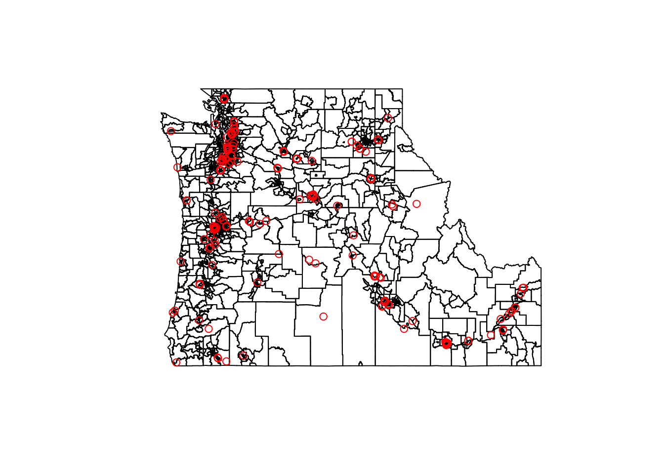

Now it’s time to find the tracts that are within 50km of a school. We can do this a few ways. First, we’ll use the st_buffer approach. We can also calculate the distance matrix between the schools and the tracts using st_distance. This adds a little more complexity as we have to then find the values that are greater than 50km. You’ll notice that st_distance returns a matrix with a row for each school and a column for each tract. This is a little clumsier to deal with, but more precise than a simple buffer.

school.buf <- landmarks.proj %>% 
  st_buffer(., dist=50000) 

school.dist <- st_distance(landmarks.proj, cejst.pnw)
dim(school.dist)

[1]  220 2571

Once we have the buffered “footprint” of the school we can use st_filter (which filters using topological relations) combined with the st_covered_by predicate to find all of the cejst.pnw tracts that are covered by the buffer. Notice that if we use the typical [] subset we get over 200 more records. This is because the latter takes all tracts with an intersection (rather than using our covered by criteria.). We can alter this to achieve the same result as the st_filter by adding the op= argument. Using the distance to the points themselves can be a more conservative way of calculating this, but takes a little more work. First we have to get a list of all of the tracts that fall within 50km (using st_is_within_distance), then identify which of those list elements are empty (i.e., no schools are within 50km), then set that as an index to subset our cejst data.

school.tracts.stf <- cejst.pnw %>% 
  st_filter(x =., y = school.buf, .predicate = st_covered_by)
school.tracts.sbst <- cejst.pnw[school.buf,]
school.tracts.sbst2 <- cejst.pnw[school.buf,, op=st_covered_by]

nrow(school.tracts.stf)

[1] 2285

nrow(school.tracts.sbst)

[1] 2512

nrow(school.tracts.sbst2)

[1] 2285

identical(school.tracts.stf, school.tracts.sbst2)

[1] TRUE

within50 <- st_is_within_distance(cejst.pnw, landmarks.proj, dist=50000, sparse = TRUE)
within50.idx <- lengths(within50) > 0
school.tracts.sbst3 <- cejst.pnw[within50.idx,]
nrow(school.tracts.sbst3)

[1] 2511

3. Make a map for both the percentage of individuals with less than a high school degree in counties within 50km and beyond 50km (i.e. make 2 maps)

We now have the full cejst dataset and a dataset that is subsetted to the tracts within 50km of a school. Plotting the HSEF values for the tracts within 50km of a school is easy enough. Just map a layer that contains all of the tracts and set it’s color to gray. Then layer the subsetted features on top. Plotting the values of HSEF for the tracts beyond 50km is a little trickier (because we haven’t created that dataset yet). We can use the index we created in the previous step to do that here. We can also use the mutate function to create an indicator variable using our index and then create a “small multiples” style map that plots the two side by side. We’ll learn more about “prettying” up these maps in the later parts of the course.

tm_shape(cejst.pnw) +
  tm_polygons(col="gray") +
  tm_shape(school.tracts.sbst3) +
  tm_fill(col="HSEF")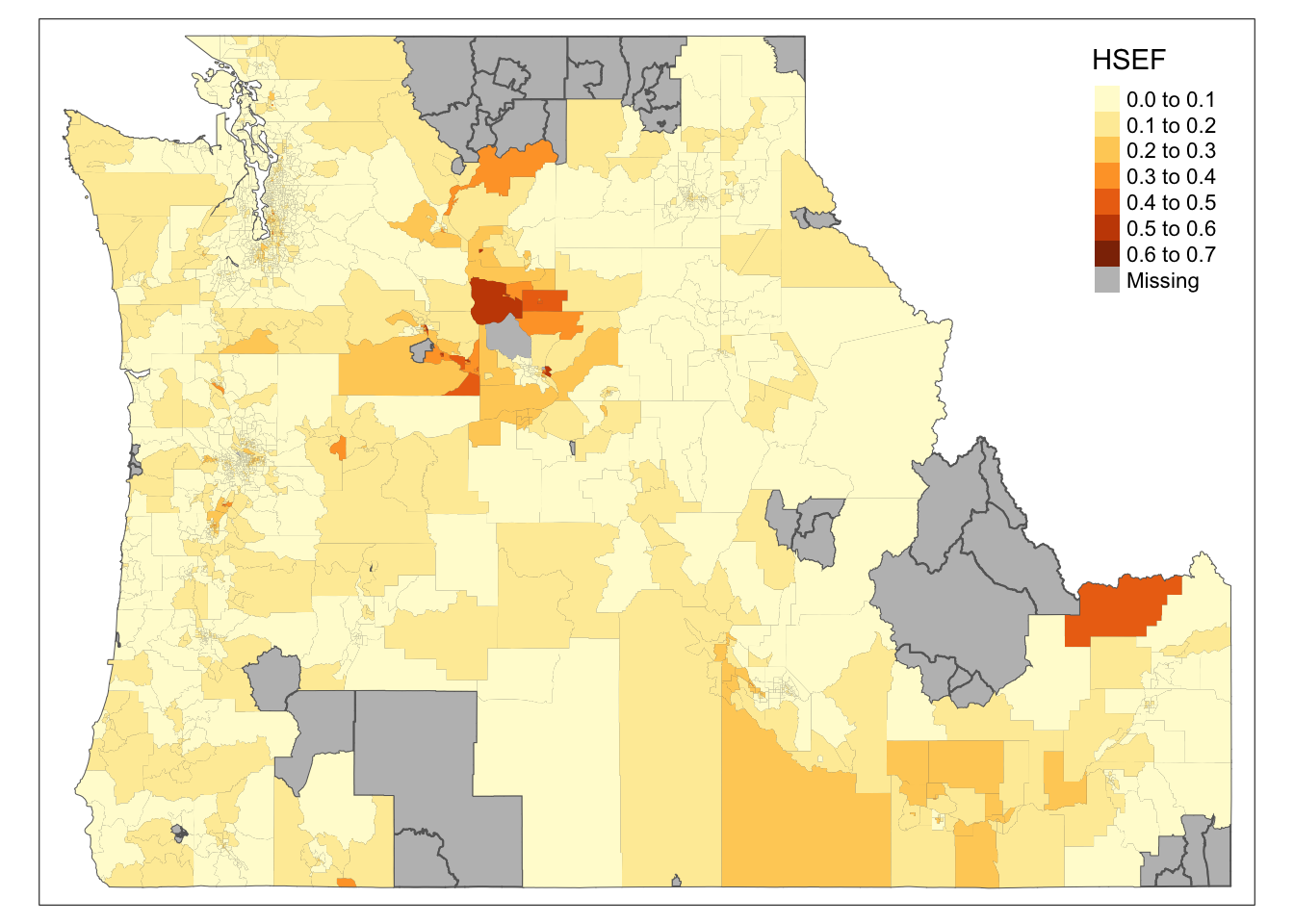

noschool.tracts <- cejst.pnw[!within50.idx,]
tm_shape(cejst.pnw) +
  tm_polygons(col="gray") +
  tm_shape(noschool.tracts) +
  tm_fill(col="HSEF")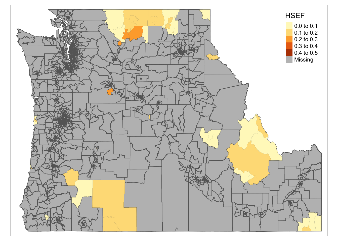

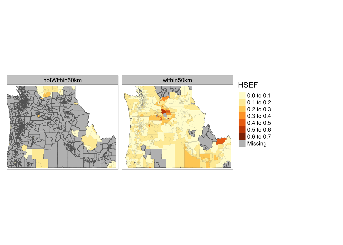
school.combined <- cejst.pnw %>% 
  mutate(., indist = if_else(lengths(within50) > 0, "within50km", "notWithin50km"))


tm_shape(cejst.pnw) +
  tm_polygons(col="gray") +
  tm_shape(school.combined) +
  tm_fill(col="HSEF") +
  tm_facets(by = c("indist"), nrow = 1)